In the earlier post, we discussed the importance of mathematics in Chemistry. We also talked about the concept of variables. In this post, we shall learn to plot the experimental data on graphs. Graphs provide a pictorial representation that is easy to comprehend.
Before we start talking about graphs, we should know the coordinate systems. These systems help us locate specific areas on the graph, and plot points accordingly.
The Coordinate System
Look at the space around you. Note the number of 90° angles you see. Almost all the walls intersect each other at 90°. We are almost always surrounded by rectangular spaces- rooms, cubicles, and offices. We have many objects in them. Consider a table lamp. If we want to specify its position in the room, we need the coordinate system. The coordinate system is a spatial reference system used to determine the location of objects. The GPS systems we use so extensively are a perfect example of the coordinate system.

The coordinate system was ideated by a French mathematician named René Descartes.
The simplest example of a coordinate system, in one-dimensional space, is the number line. The zero on the number line is considered the origin.

If point A is plotted on the number line, its distance from the origin is measured. In the figure below, point A is to the right of the origin. Thus, its value is considered to be +3. This is an example of a one-dimensional space.

In a two-dimensional Cartesian coordinate system, we have two axes, namely the x– and y– axes. The vertical y-axis is called the ordinate and the horizontal x-axis is called the abscissa. These two axes are perpendicular to each other. They intersect at the origin ‘0’ as shown below-
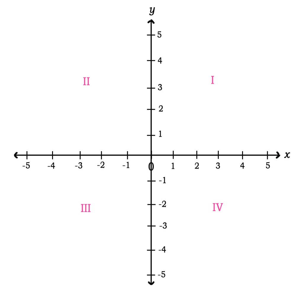
The intersection of the two axes creates 4 sections called ‘quadrants‘. Thus there are 4 quadrants namely- I, II, III, and IV.
Any point plotted in this 2D- space can be defined by two coordinates – the x– and y– coordinates. The point is represented as (x,y). The first value in the bracket gives us its x-coordinate and the second value it’s y-coordinate.

However, spaces around us are viewed in 3-dimensions. To extend the cartesian coordinate system in 3D, a third line is drawn that is perpendicular to both the x– and y– axes. These are all linear cartesian coordinate systems.
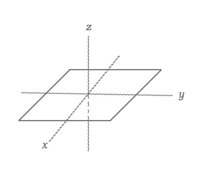
However, atoms and molecules operate in the round zone. They are NOT linear. Thus we need plane polar or spherical polar coordinates to describe them.
However, while plotting normal graphs we only need to consider a two-dimensional space. When we plot quantities like pressure, volume, or time, we know that the numerical values of these quantities are ALWAYS POSITIVE NUMBERS. Therefore, the graphs we encounter just show the first quadrant.
GRAPHS
Graphs are diagrams for data representation. It is said, ‘Pictures speak louder than words‘. Graphs are the pictorial representation of specific data. Graphs allow us to see trends, variations, and anomalies in the data recorded. They are the visual tools that allow us to grasp the data easily.
In data representation, straight-line graphs are preferred as they show the data trends very clearly. One can get results, with a specific set of values, without having to record them experimentally.
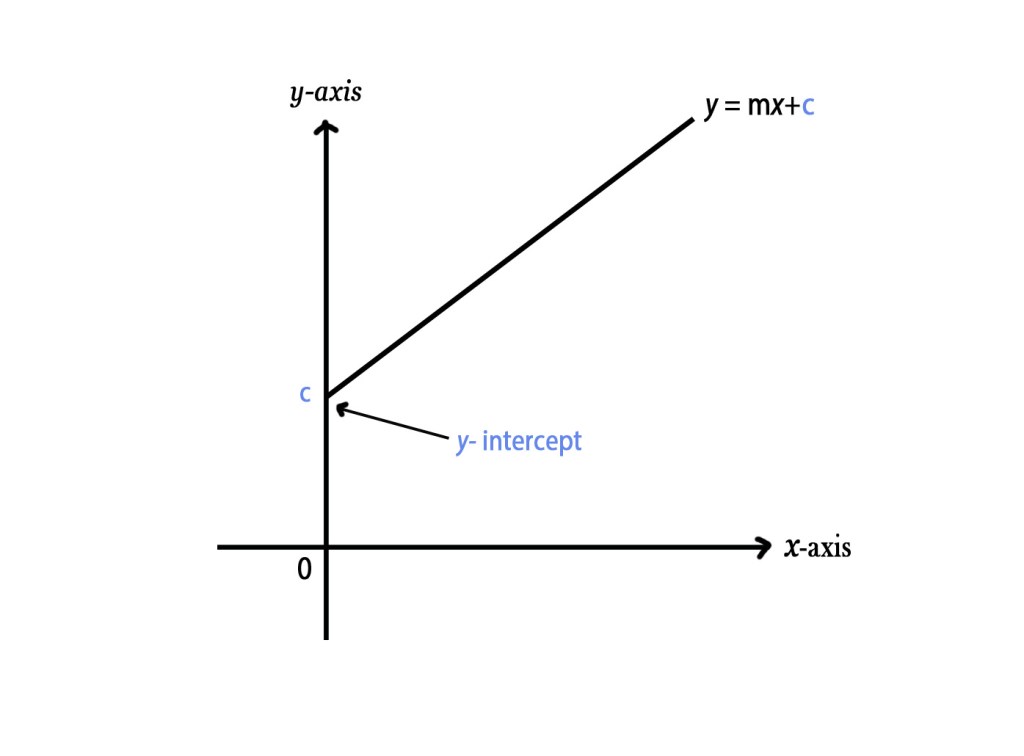
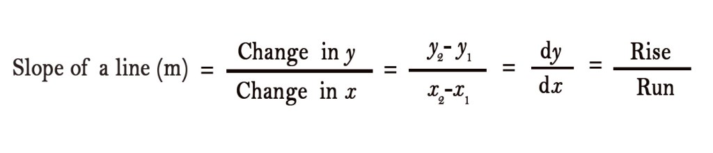
We learned in Mathematics that a straight line can be represented by the equation,
y = mx+ c, where,
x, y → variables
m, c → constants
The above equation has two variables and two constants.
The two variables – (Click here to know more about variables).
i) y= dependent variable
ii) x= independent variable
Intercepts
The point where the graph crosses the x-axis is called the x-intercept. Similarly, the point where the graph crosses the y– axes is called the y-intercept.
The pink line in the graph shown below intersects the x-axis at -3. Thus, its x-intercept = -3.
Similarly, it intersects the y-axis at +4. Thus, its y-intercept = +4.

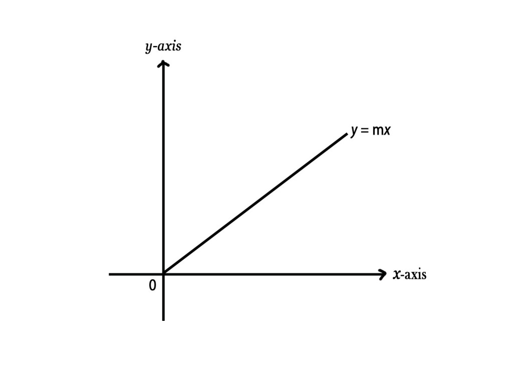
If the line passes through the origin(0), then the equation of the lines becomes y=mx, as the y-intercept, c=0. (see fig below)
The slope of the line (m)
The word ‘slope’ is derived from the Latin root ‘slupan’ meaning to slip or glide. The value of ‘m’, gives us a sense of how steep/slanting the line is.
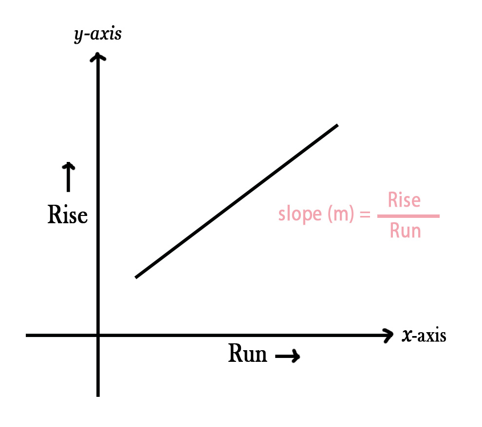
The rise is the change of coordinates along the y-axis. This difference tells us how much the line has risen above the x-axis. The run is the change of coordinates along the x-axis. It gives us the horizontal displacement of the line.
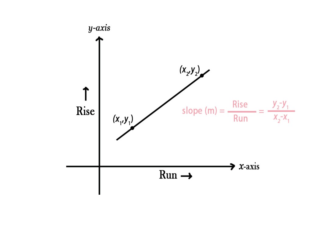
Consider any two points on a line. As shown in the graph below, the coordinates of these points are (x1,y1) and (x2,y2). (y2– y1) is the rise and (y2– y1) is the run. Dividing the rise with the run gives us the slope of that line.
So what does the slope tell us?
The slope of a line represents the change in y-value per unit change in x-value i.e. it tells us the rate of change of y with respect to change in x. The larger the magnitude of the slope, the steeper the line is, i.e. the more it approaches the vertical.
If the line is –
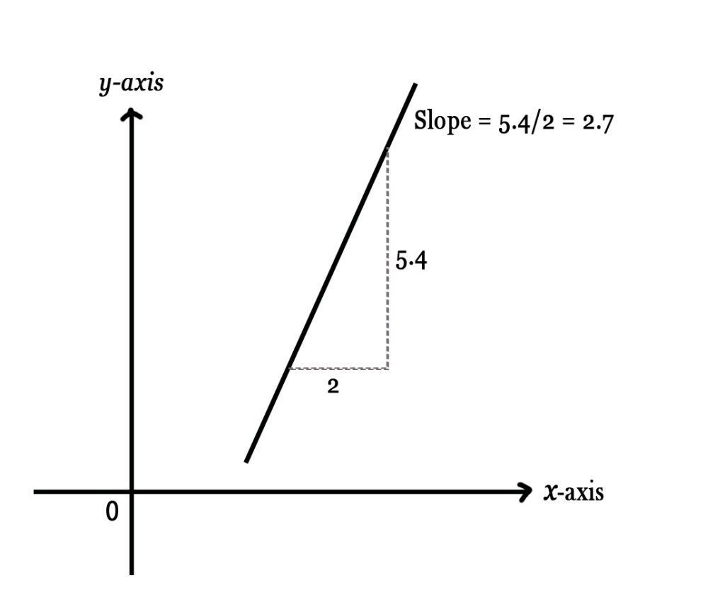
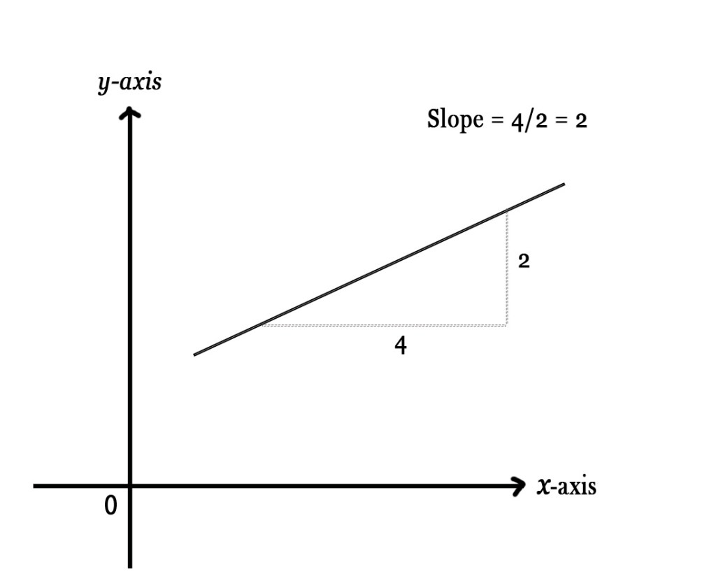
i) more vertical means y is changing faster with little progressions in x. Here, the value of the slope is comparatively more which indicates that the line is steep or less slanting. The first graph in the figure above has the maximum slope(2.7). Thus, the line is very steep.
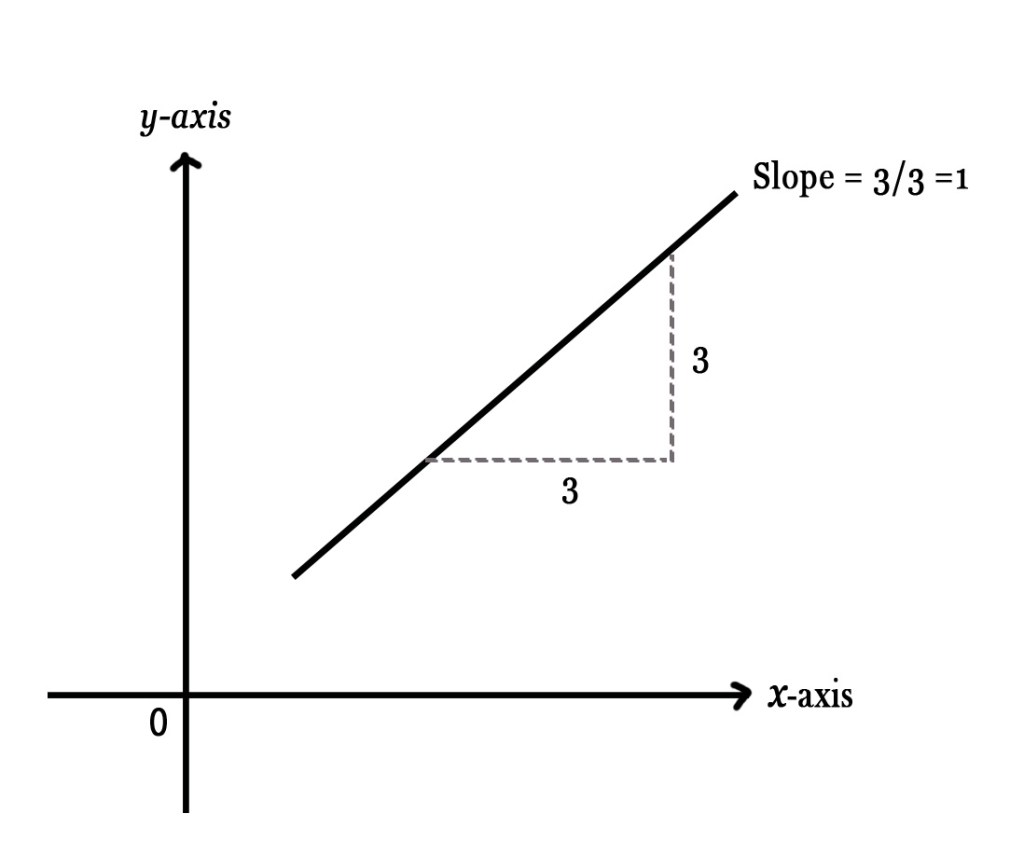
ii) more horizontal means y is changing slowly with respect to the change in x. Here, the value of the slope is comparatively less which indicates that the line is more slanting.
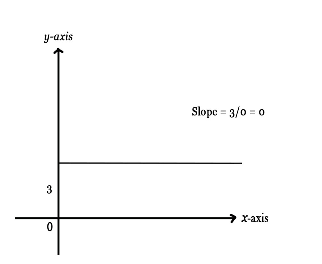
iii) if the line is horizontal, parallel to the X axis, it means the value of y is NOT changing with x. So, y2-y1 = 0, thus m= 0.Here, the slope is zero means the gradient or the rate of change is zero.
The slope can be negative, positive, or zero.
i) Going from the left end of the line to the right, if the line goes up then it’s a positive slope. It’s like going up the hill.
ii) Going from the right end of the line to the left, if the line goes down, then it is a negative slope. It’s like coming down the hill.
iii) Zero slope is like walking on a straight, flat ground.
So, the following graphs will exactly tell us how to interpret graphs-
These concepts will be useful while studying the rates of reactions where we study the rate of change of concentration of reactants with time.
Point to remember → Straight-line representation of data helps us understand our experimental data better and thus scientists always strive to get the data on a straight line.
But what if we get a curve on the graph with our experimental data values? We shall try to discuss more on this in the next post. Till then,
Be a perpetual student of life and keep learning…
Good day!
Image source –
1)https://www.montereyinstitute.org/courses/Algebra1/COURSE_TEXT_RESOURCE/U04_L1_T1_text_final_files/image014.gif
2) http://mathsfirst.massey.ac.nz/Algebra/StraightLinesin2D/Slope.html
3) By After Frans Hals – André Hatala e.a. De eeuw van Rembrandt, Bruxelles: Crédit communal de Belgique, ISBN 2-908388-32-4., Public Domain, https://commons.wikimedia.org/w/index.php?curid=2774313
