Niels Bohr brought a revolution by making necessary amendments to Rutherford’s nuclear model and later proposing his own model. The beauty of his predictions was that experimental data could easily authenticate them. Let us begin this post by studying the hydrogen atom spectra with a connection to the Bohr Model.

---

What is a spectra?

Before studying the Hydrogen spectra let us first understand the fundamental concept of a spectrum.

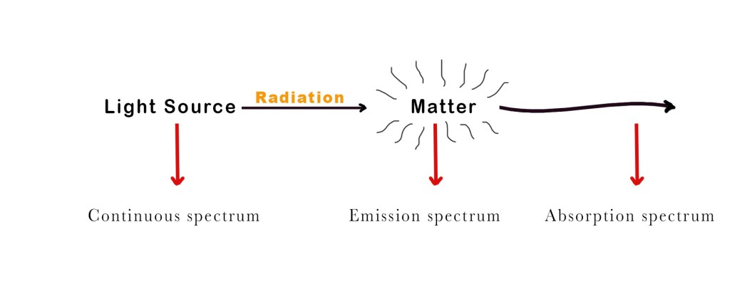
A spectrum is a chart or graph showing how light interacts with matter. There are three types of spectras –

1. Continuous spectrum – This kind of spectrum is produced by the dispersion of light. As the name suggests, this type of spectrum is continuous. There are no gaps or dark bands. Such kinds of spectra are emitted by any warm substance. Different substances emit different radiations at specific temperatures. Some examples –
   i) Iron– When a piece of iron is heated, it first glows red, then yellow and finally white. Before glowing red it emits IR rays which can be felt by our skin but these rays are not visible to human eyes.White-hot iron emits UV rays too.
   ii) Tungsten– A tungsten filament (used in a light bulb) at 2500K emits light in the visible range.
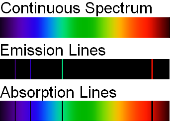
   When white light is dispersed through a prism, it separates into 7 different colours (VIBGOYR) without any gap between two consecutive colours. This spreading of the colours is called a continuous spectrum.
2. Emission spectrum – When light is shone upon a substance, it absorbs some wavelengths and emits the remaining ones. The emission spectra show us lines/bands of radiation emitted by the object under study.
3. Absorption spectrum – The absorption spectrum has dark lines/gaps that indicate the wavelengths absorbed by the substance under study.
   

Type of Substance	Type of spectrum
Hot opaque Body e.g. a dense gas/solid	continuous spectra,like rainbow of colors.
Hot transparent gas e.g. Hydrogen gas in a gas discharge tube	emission spectra- specific lines on a dark background.
Cool transparent gas(source of light continuous)	Absorption spectra – dark lines between the colors of continuous spectra.

The discreet lines in the emission spectrum occur at exactly the same wavelengths as the dark lines in the absorption spectrum.

---

H-atom spectra and the Bohr Model

According to Bohr Model , E_(n) = – R_H (Ƶ²/n²).

For H- atom in the gas phase, Ƶ=1 (as the atomic number of hydrogen is 1).

So, for H-atom, E_(n) = – R_H/n².

Using this formula let us try to find energies for different orbits in the hydrogen atom.

Note ⇒  R_H = 1.1 ×10⁷ m ^-1 =2.18 x 10^–18 J = 13.6 eV.

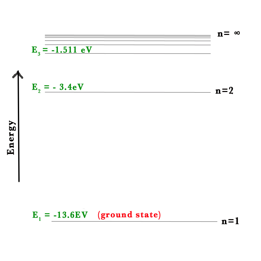
Energy for the first orbit, E₍₁₎ – the orbit closest to the nucleus, n=1-

E₍₁₎ = – R_H/(1)² = -13.6/1 = -13.6 eV.

For n=2, E₍₂₎ =- R_H/(2)² = -13.6/4 = -3.4 eV.

For n=3, E₍₃₎ =- R_H/(3)² = -13.6/9 = -1.511 eV.

Note that all values of E are negative. As the value of n increases, the value of energy also goes up (-1.511 > -13.6).

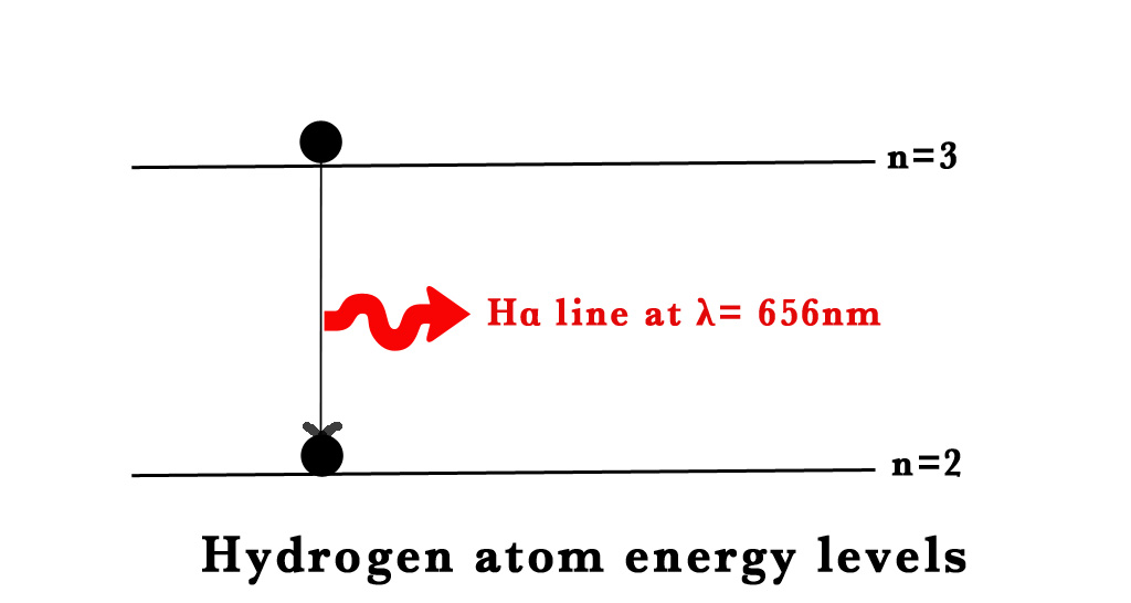
When the ground state electron in the H-atom is excited by the input of energy, it falls back down to the ground state emitting electromagnetic radiation (EMR). This phenomenon of excitation and falling back of the electrons gives rise to the atomic spectra. Lines of definite colours are observed in the spectrum. The definite colours are specific wavelengths (λ). e.g.- the red line in H- atom spectra has a λ = 656nm). These lines are unique to an element. Thus, by observing these lines we can find out the element under study.

We have already seen that ,

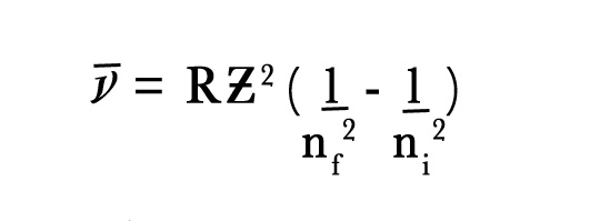
where the wave number is reciprocal of the wavelength.

∴1/λ = RƵ² {(1/n²_f – 1/n²_i)}.

The emission spectra of atomic H-atom can be divided into several spectral series, with wavelengths given by the above formula. The series is as follows –

Date of discovery	Series	Region	n1	n2
1906-1914	Lyman	UV	1	2,3,4..
1885	Balmer	Visible	2	3,4,5
1908	Paschen	IR	3	4,5..
1922	Brackett	IR	4	5,6…
1924	Pfund	Far IR	5	6,7..
	Humphrey	far IR	6	7,8..

How do we know where the emissions occur? Theoretically, we can calculate the regions using the Bohr formula and Rydberg equation.

e.g. – For the Balmer series, the electron falls from n=3 to n=2. We have already calculated the energies for these orbits above.

Thus, ΔE = E₃-E₂
= -1.511-(-3.4)
= 1.8eV
eV is NOT an SI unit. Thus, we need to convert this energy into joules, (1eV= 1.6×10^-19J).

∴1.8eV = 1.8× 1.6×10^-19J =29.76 ×10^-19J.

We know that,  ΔE = hc/λ.

∴ λ= hc/ΔE.
=(6.626 ×10^-34×3×10⁸)/29.76×10^–19.
       ≈660nm ⇒ VISIBLE RANGE⇒ This corresponds to the red line in the Balmer series.

The first series discovered was by Ångström, as he could see the discrete lines in the visible range of the spectrum. He could have discovered the series where electrons fall down to n=1 too! But unfortunately, he was using a photographic plate to detect the emissions which could only record the emissions in the visible region.

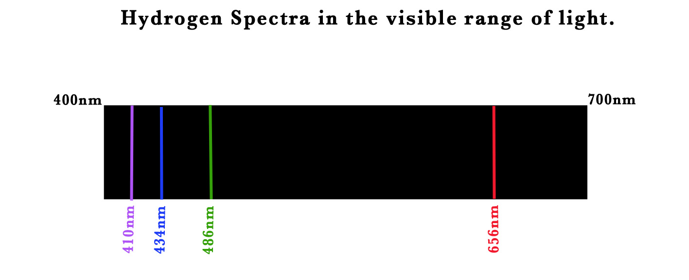
n=3 → n=2 ⇒ 410nm 
n=4→ n=2⇒ 434 nm
n=5→ n=2⇒ 486 nm
n=6→ n=2⇒ 656 nm.

The 4 lines in the Balmer series are named as  H_α ,H_β,H_𝞬 and H_δ lines.

---

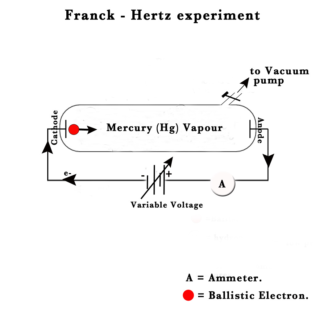
The Franck-Hertz experiment

More evidence was found in support of the Bohr Model. A year after the Bohr model was proposed, James Franck and Gustav Hertz conducted the Franck-Hertz experiment(1914).

 

In their experiment, they used a drop of mercury vapour in a vacuum tube. They sealed two electrodes, a cathode and an anode in the tube and connected them to a variable voltage source. They introduced an ammeter in the circuit. The ammeter was used to measure the electric current.

They studied the variation of current (i) with the changing voltage (v). This is what they observed –

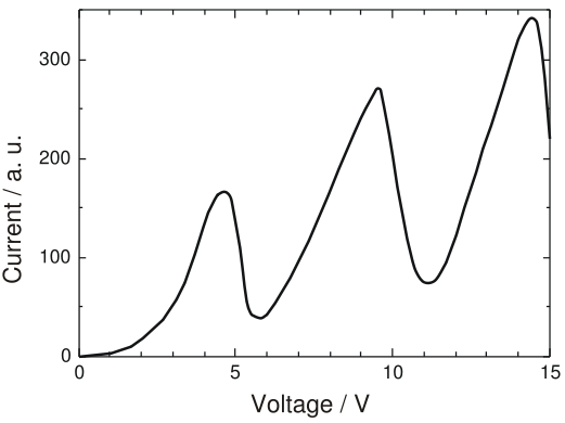
At first, they observed that they got low current at low voltage and current increased as they increased the voltage.This was as expected. However, as they kept increasing the voltage, at some critical voltage value (4.9V), the current almost dropped to zero and the tube started glowing! At this stage, they kept increasing the voltage and saw that the current  showed a rise with the increase in voltage. At another critical point (6.7V), the current dropped almost to zero again! The tube started glowing more brilliantly than before! Thus, this phenomenon showed a periodic behaviour.
The ionisation energy of mercury is 10.4 eV. The values recorded were less than the ionisation energy! So, they reasoned that electrons in the mercury atom were excited within the atom. As the glowing happens only at certain discrete values of voltage applied, the energy levels within the atom must be quantised! At the time of the experiment , both Franck and Hertz had not known about the Bohr Theory. Later they adopted this theory as a possible explanation to the phenomenon they recorded.

In 1915, Bohr published a paper noting that the measurements of Franck and Hertz were consistent with his own model for atoms. Franck and Hertz’s observed emission at 254 nm from the tube. When the calculations were done according to the Rydberg equation and Bohr model concept, the values of λ matched. Thus, this experiment showed that the energy level quantisation concept proposed for an one electron atom was true for multi electron atoms too! All atoms have quantised energy levels! The Franck-Hertz experiment thus became one of the most important experimental pillars of quantum mechanics. On December 10, 1926, Franck and Hertz were awarded the 1925 Nobel prize in Physics “for their discovery of the laws governing the impact of an electron upon an atom.”

This concept gave birth to the new world of Quantum Mechanics. Thus, Neils Bohr is correctly called ‘The Father Of Quantum Mechanics‘! Niels Bohr won a Nobel Prize in Physics in 1922.

---

LIMITATIONS OF BOHR MODEL

Though this theory was a huge step forward it had some limitations. The limitations of the Bohr model were as follows –

1)This theory could not explain multi-electron systems.

2)The theory could not explain the relative intensities of the spectral lines. Some lines were found to be more intense than others. In 1887, at Case University, Michelson and Morley (the first American to win a Nobel prize) found out that the intense spectral lines were in fact a DOUBLET! The Bohr model was incapable of explaining this hyperfine structure of the spectral lines.

3)Under a magnetic field and in an electric field, the spectral lines exhibit a splitting phenomenon.

Splitting of spectral lines in a magnetic field – ZEEMAN EFFECT.
Splitting of spectral lines in an electric field – STARK EFFECT.

Both the above effects could not be explained by the Bohr atomic Model.

These limitations proved that there was a lot more to be discovered about this small indivisible particle of matter – the atom. What were the further developments? We shall find that out in our next post. Till then,

Be  a pertpetual student of life and keep learning…

Good Day !

 

References and Further Reading –

1)http://astro.unl.edu/naap/hr/hr_background1.html

2)Lec 5 ,MIT 3.091SC Introduction to Solid State Chemistry, Fall 2010 by professor Donald Sadoway.

3)https://en.wikipedia.org/wiki/Franck–Hertz_experiment

Image source –

1)http://astro.unl.edu/naap/hr/hr_background1.html

2)https://en.wikipedia.org/wiki/James_Franck#/media/File:James_Franck_1925.jpg

3)https://en.wikipedia.org/wiki/Gustav_Ludwig_Hertz#/media/File:Gustav_Hertz.jpg

4)https://en.wikipedia.org/wiki/Franck–Hertz_experiment#/media/File:Franck-Hertz_en.svg